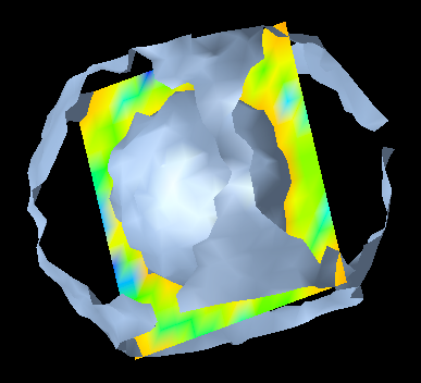
3D scalar field visualization in OpenDX: isosurfaces and a cross-section
Modern applied mathematics modelling cannot be complete without numerical simulations. Here you will learn the basics of performing these simulations efficiently and reliably. In many cases numerical models put high pressure on both software and hardware. Therefore it is important to be able to utilize the strengths of both to a maximum extent.
Syllabus
You will find the official syllabus on the course USOSweb page.
Learning materials
- TEXTBOOK:P.Krzyżanowski, Obliczenia inżynierskie i naukowe, Wydawnictwo Naukowe PWN, Warszawa, 2011 (in Polish, unfortunately)
- Textbook companion - a collection of various problems with example solutions:P.Krzyżanowski, Obliczenia naukowe (free e-book in PDF, in Polish). Online version: http://mst.mimuw.edu.pl/lecture.php?lecture=ona (in Polish, too; despite similar title, its content is almost entirely different from the TEXTBOOK). You can easily Google-translate the online version into English. The result, while not perfect, is quite readable.
- Supplementary literature in English (for those of you who do not prefer Polish yet):
- Desmond J. Higham and Nicholas J. Higham, MATLAB Guide, Second Edition SIAM, 2005
- Cleve Moler (the author of MATLAB), Numerical Computing with MATLAB SIAM, 2004, online version free for personal use
- Kermit Sigmon, MATLAB Primer, from the previous century, but still tasty and available for free!
- K.N.King, C Programming: A Modern Approach, Second Edition, W. W. Norton, 2008. Excellent source on basic and advanced programming in C language.
Grading rules
The final grade will be a weighted mean of the mid-term exam (May 12th) with weight 1/3 and of the final exam (TBA) with weight 2/3. You need to earn 50% of the total to pass. Both mid-term and the final exam will consist of several scientific computation problems to be solved a vista in the computer lab.
Each week you will be assigned some homework during the classes (only a short reminder will be posted online). Please do it, and in case of difficulties turn to my office for discussion. You will not get any extra points for your homework done but the experience says that those who do homeworks routinely score much better at the exam...
The contents of 2014/15 edition
- Introduction to scientific computing. An overview of tools. Symbolic vs. numerical calculations. Introduction to MATLAB/Octave scientific computing environment. Why is it better to avoid loops? See also: TEXTBOOK, Sections 1, 2 and 3. Homework: implement matrix-matrix multiplication using nested loops and see if this runs faster than
A*B - Using matrices and solving various linear algebra problems (systems, least squares, eigenvalues, etc.) in MATLAB/Octave. Animal breeding or the art of asking right questions. The easiest implementation is usually not the one you will be satisfied with. Writing functions and scripts in MATLAB/Octave. See also: video guides listed below and TEXTBOOK, Section 5. Homework: use all three (four?) approaches to see if you get the same results. Which is the fastest? Use artificial data X,Z,D,P. Try both small and big n. Extra homework: make your function work with data stored in a spreadsheet format (e.g. Excel or CSV).
- Solving nonlinear equations in MATLAB/Octave. Additional input and output parameters to
fsolve. Stopping criteria and computing the condition number (see TEXTBOOK, the beginning of Chapter 7.6). Chandrasekar equation solver: avoiding loops, precomputing, using global variables. Timing your code. See also: TEXTBOOK, Example 7.6.2. Homework: time our Chandrasekhar solver withfsolvenonlinear solver and verify if the depenedence is N3. Experiment with various values of c and derive the dependence of the cost on c. - READING: Newton's method with Jacobian update every k iterations for more efficiency. Optimization with constraints in Octave:
glpk,qp,sqp. Fitting reaction parameters or why should we care for more than computational effort only. Which of best fits is the best? Homework: time our Chandrasekhar solver withfsolvenonlinear solver vs. our implementation of the Newton's method. Experiment with various values of k. Extra homework: time both solvers in both MATLAB and Octave and judge if JIT compiler helps.Homework: compute condition numbers of all least squares problems we solved. How would you assess the conditioning of the nonlinear least squares fitting? - Solving ODEs in Octave with
lsode(MATLAB has different functions and slightly different syntax, but also a very good manual to start with, if you have to). Tuning ODE solver's working parameters and why this is more art than science. Van der Pol equation: solution and visualization. Homework: Examine very long time behaviour of the norm of the solution to Van der Pol equation, i.e. |y(t)|2+|y'(t)|2. What happens when epsilon=0? Aren't you surprised? How can you verify if you obtain correct results? Extra homework: write your own functionodesolvewith uniform syntax that wil work equally well in both MATLAB and Octave (so that the user will get an ODE solver which is compatible with both environments). Depending on whether it was called within Octave or MATLAB,odesolvewill use an appropriate solver (lsodein Octave). Ensure the user can always pass as the right hand side a function of the form F(t,Y) - both in Octave and in MATLAB. Think about a consistent set of options to tune the behaviour of the underlying solver(s) without additional knowledge of internal details ofodesolve. - Sparse matrices: how to create and use them. Solving systems with sparse matrices: direct factorization (
\) or iterative methods (pcg,pcr,gmres)? Preconditioning. 1D laplacian as a sparse matrix. Creating 2D Laplacian on uniform mesh usingkron. Homework: read, how to implement nonzero boundary conditions to our diffusion equation solver. - Various plotting tools for 1D and 2D real-valued functions (e.g
plot,semilogy,mesh,contour, etc.) Graph annotation. Why ill-designed plots can hurt you. More on plotting: TEXTBOOK, Chapter 6. Finite difference scheme for diffusion equation: 2D case with constant diffusion. Caution: there are much more efficient ways to solve diffusion equation. (They, however, require additional knowledge we cannot afford). Implementation and visualization in Octave (2D case). Implement 3D diffusion as described and check experimentally how large problems you can solve on your computer. Compare with 2D case. Extra homework: read the rest of the diffusion equation chapter and learn how we can significantly improve the performance of our solvers in both 2D and 3D as well! - Tentative:
- Implementing GeneRank solver (see TEXTBOOK, Example 7.3.2). Homework: Finish your implementation and test on compatible data. Real data will be provided here (soon).
- Midterm May 12th, 2015. You may check your solution against example solutions (from 2014).
- Introduction to programming numerical algorithms in C. Recommended book on C: K.N.King C Programming: A Modern Approach Homework: In order to verify the solver, use a problem with a priori known solution: try (a) u(x,y) = x(x-1)y(y-1) (b) u(x,y) = sin(pi*x)*sin(pi*y) on a unit square. In both cases set the right hand side equal to the laplacian of the accurate solution and then inspect visually if you get similar solutions from the solver. Extra homework: check how the error (the maximum absolute value of the difference between the accurate and computed soultion) behaves with the number of nodes increases: N = 10, 20, 40, 80, ... You should observe essentially no error(!) in case (a) - can you explain why? - and quadratic decrease in (b). How many little bugs have you spotted in your code with the help of these two testcases?
- Using C with external libraries. Mixing C code with Fortran77. Examples of numerical libraries: BLAS, LAPACK, ATLAS, MKL, ACML, GSL, .... Interfacing C code with (optimized) BLAS and with GSL.
- Modern computer architectures. Processor internals: cache, pipelining, multicore, vector registers.
- Code optimization. Amdahl's law and its variations. Compiler switches. OpenMP. Recommended book on code optimization: Goedecke, Hoisie, Performance Optimization of Numerically Intensive Codes, SIAM, 2001. See also TEXTBOOK, Chapter 11 for a brief intro.
- Scientific visualization. Common mistakes. Standard ways to deal with (mutlidimensional) data fields. Paraview and its data format(s). Regular grid data visualization in Paraview. See TEXTBOOK, Part 4 for more examples.
A collecion of video guides to MATLAB and Octave
For Octave, Paul Nissenson from UC Irvine, has created a series of Octave tutorial videos, all to be watched on YouTube. Enjoy!
You can follow many online videos which cover various usages of MATLAB and come directly from the MathWorks, the producer of MATLAB. Many of them are still free to view. I recommend you to start with:
- Getting Started with MATLAB
- Writing a MATLAB program
- Importing data from files
- MATLAB fundamental classes
- Basic plotting functions
- Programming and developing algorithms
You can find even more videos on MATLAB YouTube channel. You can find more links to demos, books and tutorials on Mathworks' web page with learning resources.